
Mastering Stream Processing - Introduction to windowing.
by Bill Bejeck
Stream processing is the best way to work with event data. While batch processing still has its use cases, and probably always will, only stream processing offers the ability to respond in real-time to events.
But if we zoom in, what does it look like to respond to events? By now, I’m sure you’re familiar with the oft-quoted fraud scenario - a person with nefarious intent gets a hold of an unaware consumer’s credit card number. Still, due to the bank’s responsiveness processing system, the fraudulent charge gets declined.
Other uses of stream processing require an immediate response but are not tied to one single event. Consider monitoring the heat of a manufacturing process; if the average temperature reaches a certain threshold in a given period, then the monitoring process should generate an alert. But this isn’t about one temperature spike. It’s about a consistent upward trend. In other words, what are the temperature readings doing during a fixed period?
I’m talking about windowing in event streams, if you have not guessed by now. While aggregations (an aggregation is a grouping of events by a common attribute) are a vital tool to leverage an event stream, an aggregation over all time doesn’t shed any light on specific periods of activity. Consider the following illustration:
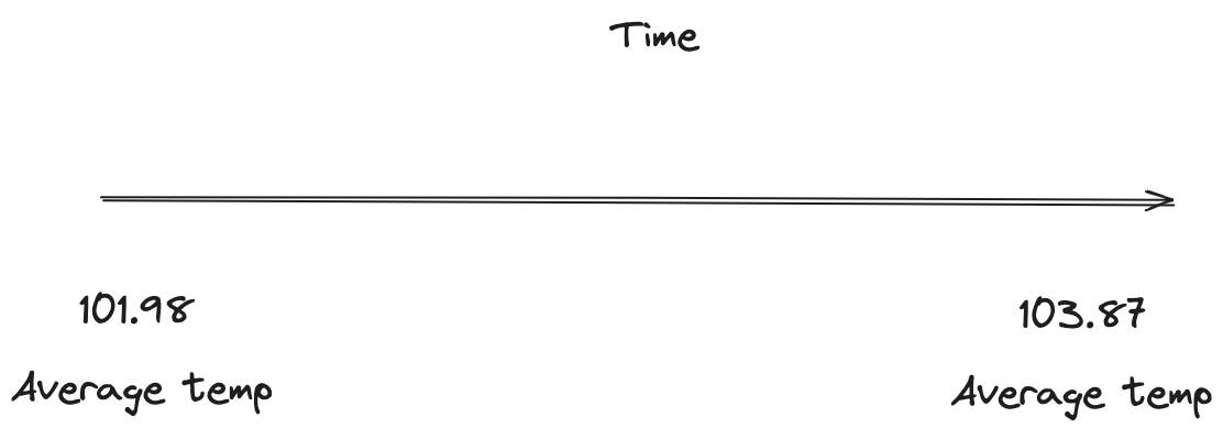
Over time the average temperature reading has increased some over time, but it doesn’t tell the whole story. Now let’s take a look at capturing the average temp readings over specific intervals:
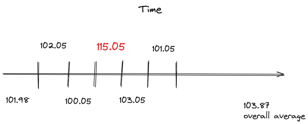
Now by getting readings at specific intervals (windows) you can spot the issue with a large jump in the average value.
This is not to say that an aggregation over all time isn’t helpful, but that, in many cases, you’ll want to aggregate over specific intervals. In other cases, you’ll want an aggregation not defined by fixed time boundaries but by behavior, e.g., session windows whose boundaries are based on periods of inactivity. We’ll get into session windows in a post later in the blog series.
This blog post marks the first in a series about windowing in the two dominant stream processing technologies today: Kafka Streams and Flink, specifically Flink SQL). It’s important to note that the point of this blog series is not a direct comparison between the two APIs. Instead, it is a resource for windowed operations in Kafka Streams and Flink SQL. While comparing the two in a competitive analysis is natural, it’s not the main focus here.
The blog series will discuss:
-
The different types of windowing, semantics, and potential use cases.
-
Time semantics
-
Interpretation of the results
-
Testing windowed applications
I will assume basic familiarity with Kafka Streams and Flink SQL, so the examples will start by covering windowing.
But before we get into windowing, let’s discuss how Kafka Streams and Flink SQL structure windowing applications. We’ll only cover this level of detail in this initial post, and subsequent ones will assume knowledge of how to assemble the program and focus on the windowing aspect.
Kafka Streams windowing
You’ll need to specify an aggregation to do any windowing in Kafka Streams. Aggregations are a function that combines smaller components into a large composition, clustered around some attribute, which in Kafka Streams will be the key in the key-value pairs. You can also perform a reduce, a specialized form of aggregation, since a reduce operation will return the same type as its input components. Generally, an aggregation can return a completely different value from the inputs. But since windowing operates the same for either a reduce or aggregation will use an aggregation for our examples throughout the blog series.
A Kafka Streams windowed aggregation
KStream<String,Double> iotHeatSensorStream =
  builder.stream("heat-sensor-input",
    Consumed.with(stringSerde, doubleSerde));
iotHeatSensorStream.groupByKey()
      .windowedBy(<window specificatation>)
        .aggregate(() -> new IotSensorAggregation(tempThreshold),
         aggregator,
         Materialized.with(stringSerde, aggregationSerde))
         .toStream().to("sensor-agg-output",
           Produced.with(windowedSerde, sensorAggregationSerde))
Let’s walk through the essential points of setting up the Kafka Streams window aggregation:
-
The first step is to group all records by key; this is required before performing any aggregation. Here you’re using KStream.groupByKey which assumes the underlying key-value pairs have the correct keys needed for clustering together. If not, you could use the KStream.groupBy function where you pass a KeyValueMapper instance that maps the current key-value pair into a new one which allows you to create a new key suitable for the aggregation grouping. Note that changing the key for a group-by will lead to a re-partitioning of the records.
-
You are specifying the windowing - we’ll cover the specific types in later posts.
-
Point three is where you’re specifying how to aggregate records. The first parameter is an Initializer represented as a lambda function, which provides the initial value. The second parameter is the Aggregator instance, which performs the aggregation action you specify. Here, it’s a simple average and tracking the highest and lowest values seen. The third parameter is a Materialized instance specifying how to store the aggregation. Since the value type differs from the incoming value, you must provide the appropriate Serde instance for Kafka Streams to use when (de)serializing records.
-
The final point is where you provide the Serde instances for producing the results back to Kafka. The key Serde is a different type as Kafka Streams wraps the incoming record key in a Windowed instance.
What’s not apparent from this aggregation example is where the timestamps for the window are. But there’s a big hint in the explanation of the aggregation example. At point four of the aggregation description, Kafka Streams wraps the original key in a Windowed object.
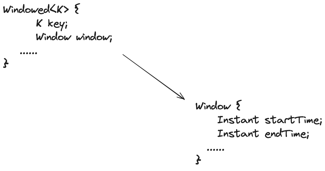
As shown in this illustration, the Windowed object contains the original key and the Window instance for the aggregation values. The Window object has the start and end time for the aggregation window. It doesn’t contain the window size, but you can easily calculate the size by subtracting the start time from the end. We’ll cover reporting and analyzing the aggregation window times in a follow-on blog post.
Wrapping the original key in a Windowed object changes the type, meaning you’ll have to update Kafka Streams on serializing the results. Fortunately, Kafka Streams provides the WindowedSerdes utility class making it easy to get the correct Serde for producing results back to Kafka:
Using the WindowedSerdes class to get a Serde for Windowed keys
Serde<Windowed<String>> windowedSerde =
        WindowedSerdes.timeWindowedSerdeFrom(String.class,
                                              60_000L
                                            );

KStream<String,Double> iotHeatSensorStream =
  builder.stream("heat-sensor-input",
    Consumed.with(stringSerde, doubleSerde));
  iotHeatSensorStream.groupByKey()
         .windowedBy(<window specificatation>)
         .aggregate(() -> new IotSensorAggregation(tempThreshold),
              aggregator,
               Materialized.with(stringSerde, aggregationSerde))
         .toStream().to("sensor-agg-output",
           Produced.with(windowedSerde, sensorAggregationSerde))
-
The class type for the original key
-
The size of the window in milliseconds
-
Providing the Serde for the Windowed key
So, by using the WindowedSerdes class, you provide the proper deserialization strategy for Kafka Streams to produce windowed results back to Kafka. Producing windowed results to a topic implies downstream consumers will know how to handle the windowed results as well. We’ll cover that situation in a later blog on reporting in a subsequent post in this series.
Now, let’s move on to Flink SQL aggregation windows.
Flink SQL windowing
Flink offers windowing for event stream data as windowing table-valued functions (TVF). The Flink TVFs implement the SQL 2016 standard Polymorphic Table Functions (PTF). In a nutshell, PTFs allow for user-defined functions on a table that returns a table.
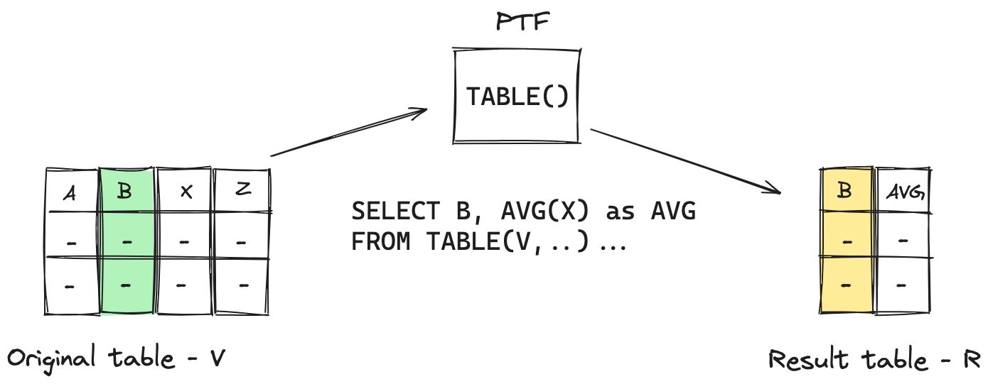
The exciting thing about PTF is that the schema of the table returned by the function is dynamic; it’s determined at runtime by the function output. So, the PTFs enable windowing and aggregation functions on existing tables, precisely what we get with the Flink SQL windowing. The windowing TVFs in Flink replace the now deprecated Group Window Functions. Window TVFs provide more powerful window-based calculations like Window TopN and Window Deduplication.
Now, let’s move on to how you execute a windowed aggregation in Flink SQL. As with the Kafka Streams example, we’ll review the structure of a windowed aggregation, with specific window implementations covered in later posts.
Structure of Flink SQL windowed aggregation
SELECT window_start,
       window_end,
       device_id,
       AVG(reading) AS avg_reading

FROM TABLE(
           <Window Function> (
                              TABLE device_readings,
                              DESCRIPTOR(ts),
                              INTERVAL '5' MINUTES,
                              [INTERVAL '10' MINUTES]
                            )
           )
GROUP BY window_start,
         window_end,
         device_id
Here’s the breakdown of the query:
-
Selecting the columns and the aggregation using the Flink SQL AVG function and providing a descriptive name; these columns form the schema of the returned table.
-
The TABLE function
-
Here, you give a specific window function, either HOP, TUMBLING, or CUMULATE. Support for a SESSION type is coming soon. We’ll cover the specific types in later posts.
-
Next are the parameters for the window function, starting with the table to use for the input
-
The DESCRIPTOR is the time attribute column the function uses for the window.
-
Depending on the window function, the following 1 or 2 parameters determine the window advance and size or just the size.
-
As with standard SQL aggregate functions, we need the same columns in the GROUP BY clause in the SELECT clause.
Flink SQL inserts three additional columns into windowed operations, window_start, window_end, and window_time. Flink SQL determines window_time by subtracting 1ms from the window_end value.
This concludes our introduction to the structure of windowing applications in Kafka Streams and Flink SQL. In the next edition, we’ll cover hopping and tumbling windows.
Resources
Subscribe via RSS